Local gravity field models for the Moon
Sander GoossensIn addition to global gravity field models of the Moon such as GRGM1200A, our group has also developed local models of the lunar gravity field using GRAIL data. Global gravity models are often described using spherical harmonics. To express features at small scales in spherical harmonics, an expansion up to high degree and order is needed. However, spherical harmonics have global support, which means that they are defined over the whole globe and thus also express signal over the whole globe. In the case that the data used to determine the spherical harmonic coefficients are geographically variable with less dense coverage in some areas compared to others, this can pose a problem: at small scales, the signal in areas with fewer data points can be too large, or the signal can show strong, unrealistic oscillations. This can be overcome with regularization, or constraints, i.e. introducing additional information to stabilize the system. For gravity field determination, the regularization of choice is often the Kaula rule, which biases the coefficients towards zero with the expectation that they follow a power law. This suppresses spurious signal but can also result in the underestimation of peak-to-peak gravity values. Local methods can help alleviate this: their support is local, which means they only have a signal in a well-defined area. Local methods have been used successfully for the determination of gravity field models on the Moon, Mars, Venus, Jupiter's moon Ganymede, and of course Earth.
Method
Our local solutions using GRAIL data are expressed in gravity anomalies, which are deviations with respect to a background global gravity field model. We assign a gravity anomaly value to a grid cell of chosen size, and then use the GRAIL Ka-band range-rate (KBRR) to estimate the anomaly values. Our approach uses short arcs that only span the area of interest. We use only KBRR data and we use the parametrization of Rowlands et al. (2002)1 to estimate 3 out of the 12 parameters that describe the baseline between the two satellites. After the orbits over the area of interest have been re-determined using this baseline approach, we generate the partial derivatives of the KBRR measurements with respect to the gravity anomalies. These partial derivatives are then accumulated into normal equation systems.
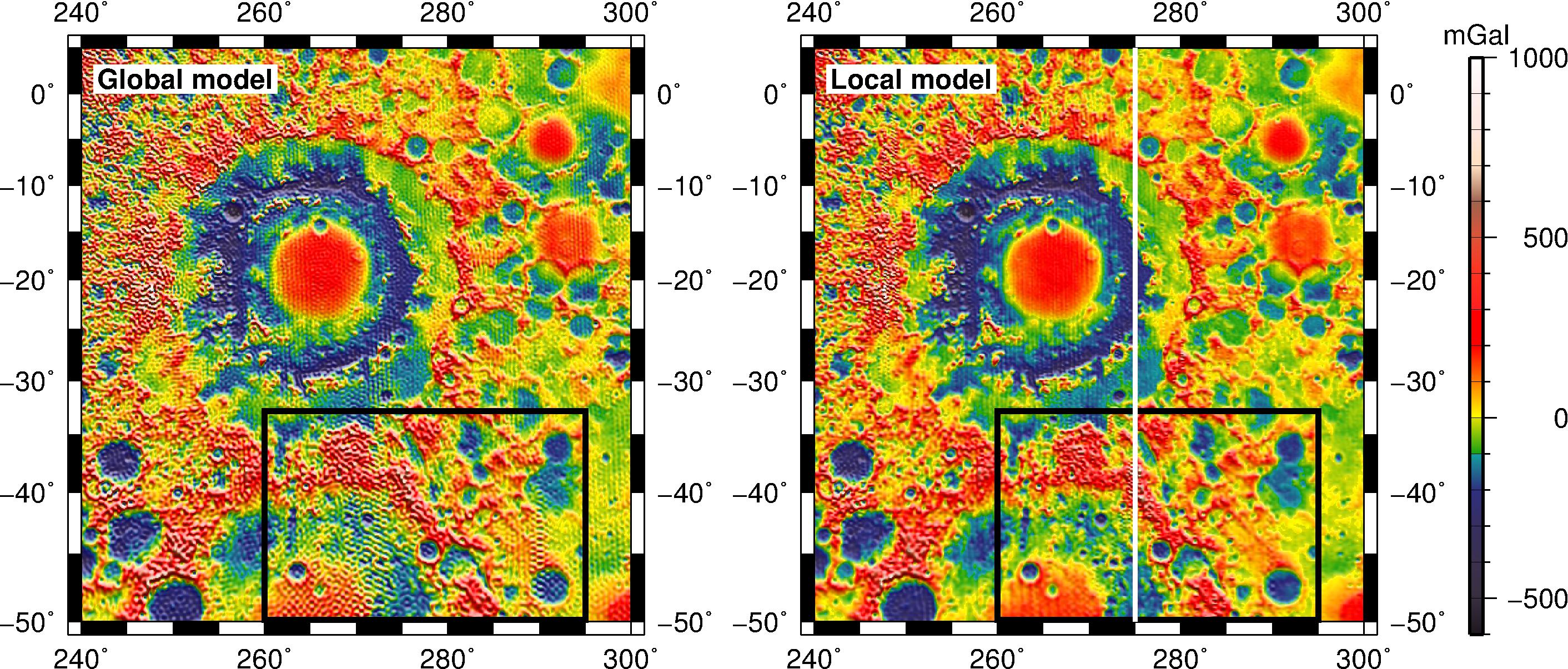
Figure: Gravity anomalies from a global (left) and local (right) model for the Mare Orientale area5. Stripes are clearly visible in the global model (note especially the area in the black box). The local solution has a mixed-resolution: 1/6 by 1/6 degree west of the white line, and 1/10 by 1/10 degree east of the white line, showing that the local grid can easily be adapted, following data coverage. This division was chosen because the lowest altitude data were taken east of the white line.
When we estimate the gravity anomalies we make use of constraints as well. The reasons are in this case not to suppress spurious signal or to counter-act varying geographical data coverage (because this is effectively taken care of by our choice of local parameters such as gravity anomalies, and the grid cell size), but to smooth the solution. We apply neighbor smoothing2,3 to the solution which effectively means that each anomaly should have its value close to that of its most direct neighbors. We assume a correlation distance so that anomalies close are more likely to have similar values than two anomalies separated geographically. Furthermore, we found4 that this works best when the constraint is applied to the total anomaly (i.e., the adjustment + start value), not just to the adjustment. Stripes occur in the solutions along orbital tracks, and for the global solutions in spherical harmonics, the applied Kaula rule does not smooth in a particular direction. The neighbor smoothing ensures that differences between neighboring cells do not change too much.
Solutions
We have applied our local analysis to several areas on the Moon: the south pole4, Mare Orientale5, and several other areas of interest. The goal is to eventually generate solutions for map that cover the whole of the Moon.
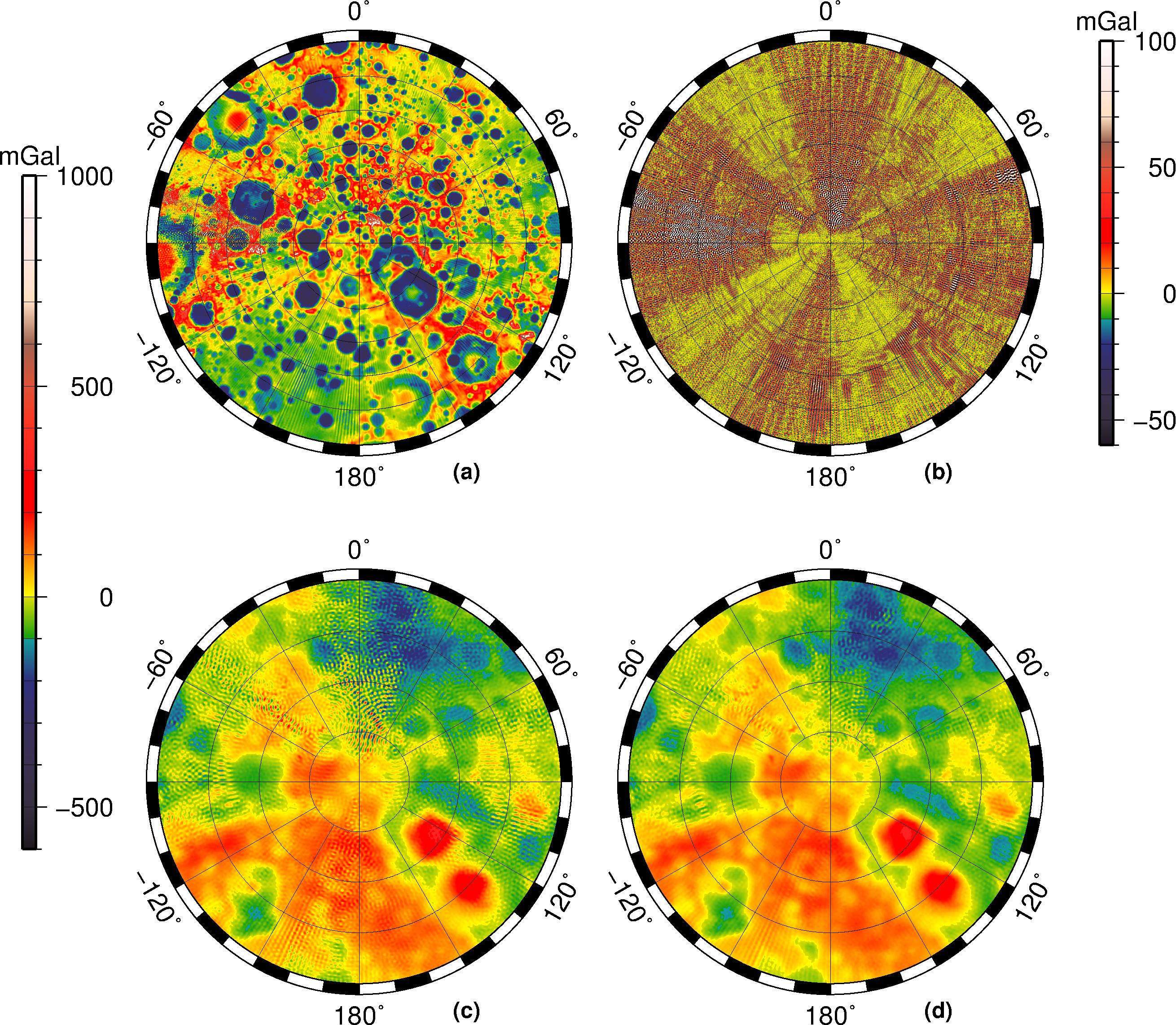
Figure: Local solutions for the south pole4. The local solution (a) and adjustment (b) are shown at the top. The bottom has Bouguer anomalies for the global model (c) and the local model (d). The local Bouguer anomalies show fewer stripes. Taken from Goossens et al. (2014)4.
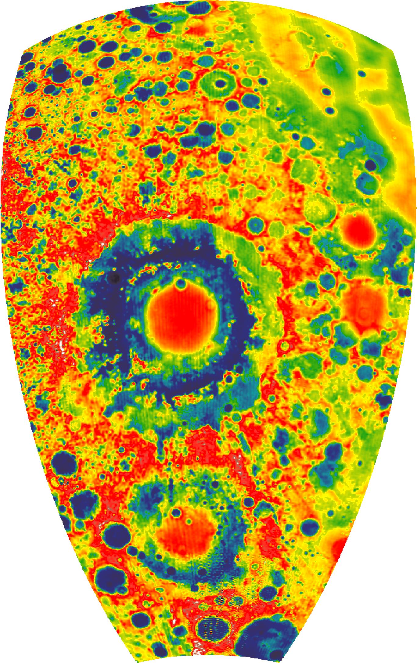
Boundary effects often arise in local methods: data close to the edges of the chosen grid are also affected by anomalies outside of the grid that are not estimated. We have investigated this by generating solutions that partly overlap. The differences between such overlapping solutions occur mostly within a few degrees of the boundaries of each separate grid, which makes us confident that we can stitch together a map by carefully generating solutions for grids with a 5 degree overlap. Such an composite example is shown in the solution for the strip of the Moon that includes Mare Orientale.
Correlations with topography
Our local solutions are expressed in gridded gravity anomalies and these maps can be readily used for analysis. However, the preference in geophysics is to use spherical harmonics. Moreover, when computing the Bouguer correction to control for the effects of topography by subtracting the gravity-from-topography from the estimated free-air gravity, both gravity-from-topography and free-air gravity have to have the same resolution. In such a case, one has to work with spherical harmonics, or a resolution in spectral space rather than in the spatial sense. If Bouguer gravity is not constructed by subtracting spherical harmonic expansions, one could account for either too much topography (if topography has better resolution than gravity, which is normally the case) or too little (if it is the other way around). For example, Bouguer gravity could show craters that do not show up in the free-air but do show up in the topography. This can give the impression of "better resolution" but one is really only looking at the negative of the gravity-from-topography (since Bouguer is computed as free-air minus gravity-from-topography). 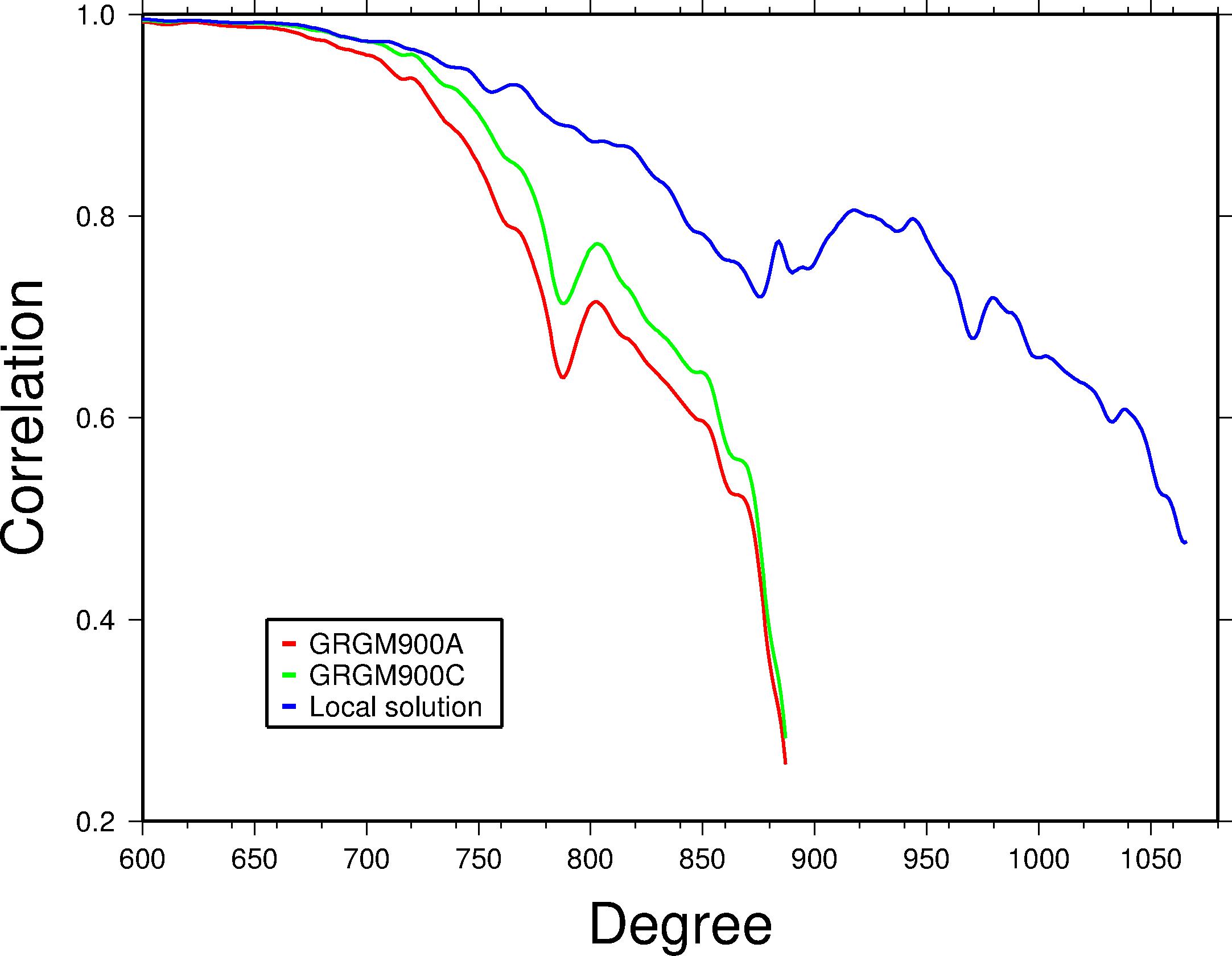
To prevent this, we transform our gridded gravity anomalies into spherical harmonics using a spherical harmonic transform based on Gauss-Legendre quadrature. This allows us to express the anomalies in spherical harmonics. This also allows us to generate the proper Bouguer solutions, and to compute correlations between our local solution and topography. We have shown that we improve correlations with topography consistently for our local solutions, making them thus suitable for geophysical analysis at the highest resolution.
References
1Rowlands, D., Ray, R., Chinn, D., and Lemoine, F.G. (2002), J. Geod., 76(307), doi:10.1007/s00190-002-0255-8
2Rowlands, D. D., Luthcke, S.B., McCarthy, J.J., Klosko, S.M., Chinn, D.S, Lemoine, F.G., Boy, J.-P., and Sabaka, T.J. (2010), Global mass flux solutions from GRACE: A comparison of parameter estimation strategies—Mass concentrations versus Stokes coefficients, J. Geophys. Res., 115, B01403, doi:10.1029/2009JB006546.
3Sabaka, T. J., Rowlands, D.D., Luthcke, S.B., and Boy, J.-P. (2010), Improving global mass flux solutions from Gravity Recovery and Climate Experiment (GRACE) through forward modeling and continuous time correlation, J. Geophys. Res., 115, B11403, doi:10.1029/2010JB007533.
4Goossens, S., Sabaka, T.J., Nicholas, J.B., Lemoine, F.G., Rowlands, D.D., Mazarico, E., Neumann, G.A., Smith, D.E., and Zuber, M.T.
(2014), High-resolution local gravity model of the south pole of the
Moon from GRAIL extended mission data, Geophys. Res. Lett., 41,
3367–3374, doi:10.1002/2014GL060178.
5Zuber, M. T., et al. (2016), Gravity field of the Orientale basin from the Gravity Recovery and Interior Laboratory Mission, Science, Vol. 354, Issue 6311, pp. 438-441, doi: 10.1126/science.aag0519