Mercury Gravity Field Models from Line-of-Sight Data and Estimation of Lithospheric Properties
Sander Goossens
We provide additional information to our paper "Estimation of Crust and Lithospheric Properties for Mercury from High-Resolution Gravity and Topography", published in The Planetary Science Journal (Goossens et al., 2022, Planet. Sci. J. 3 145, doi:10.3847/PSJ/ac703f). We provide an appendix to the paper, that contains a section on the admittance model used, and additional figures that are referred to in the paper. We provide three gravity field models of Mercury, expressed in spherical harmonics of degree and order 180. In addition, we provide the results of our admittance analysis for 4 different areas. See the “Data” section for the files.
Mercury Gravity Field Models
We base our models on an analysis of line-of-sight (LOS) data: we have transformed Doppler tracking data from the Deep Space Network to the MESSENGER spacecraft into LOS accelerations. By transforming the observational equations in the same manner, we can then estimate a gravity field expressed in spherical harmonics from these data. LOS data have the advantage that they are more sensitive to small-scale features, as shown in Figure 1: the signal generated by a gravity anomaly at the surface is narrower for LOS data when compared to Doppler data, and that means that smaller features can be described with more details, as they will be less blurred.
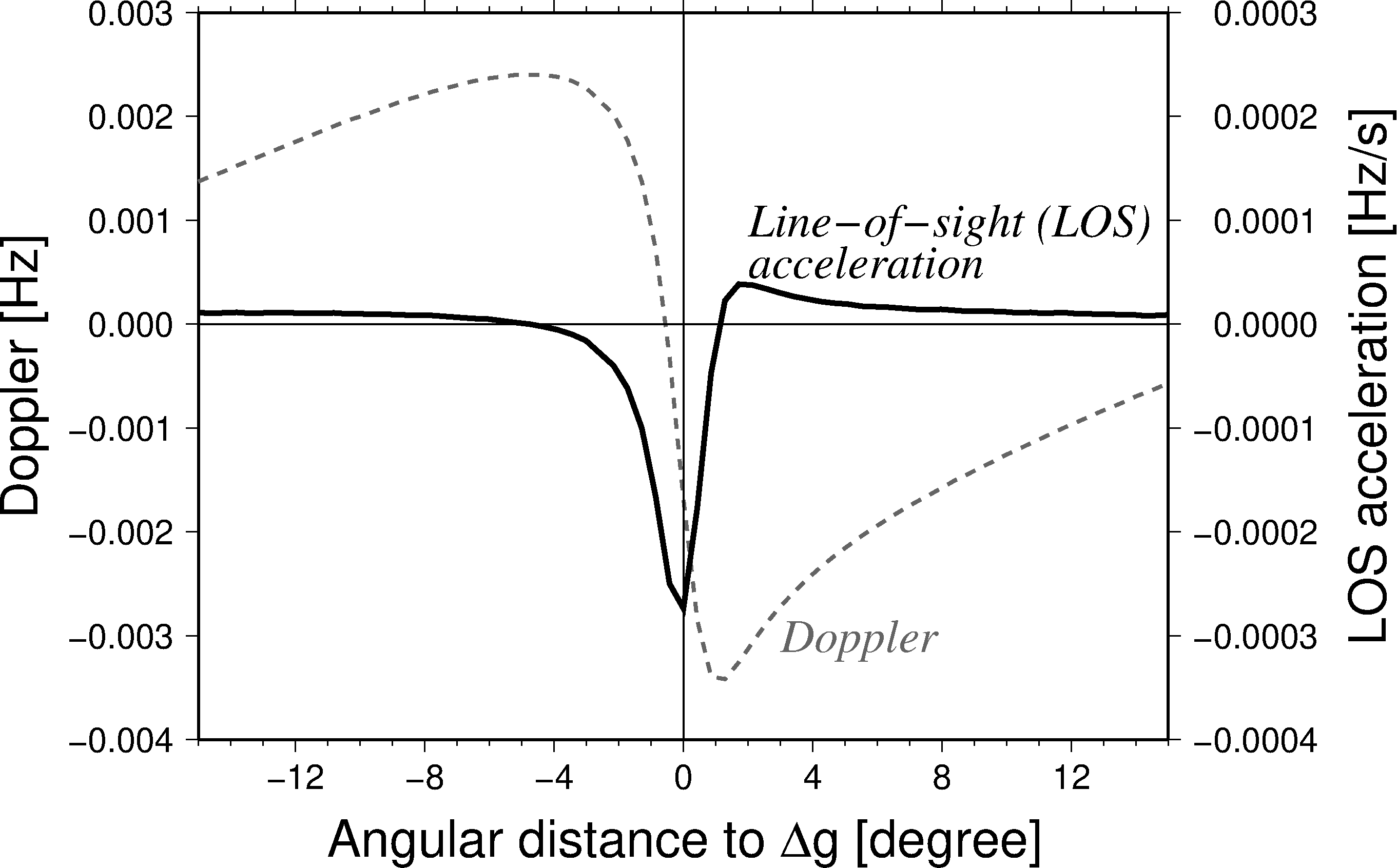
Figure 1. Influence of a 1° by 1° gravity anomaly Δg of 10 mGal on normal Doppler data and on line-of-sight (LOS) accelerations.
We show gravity field models based on normal Doppler data (denoted “Standard model”) and based on the LOS data (“LOS model”) in Figure 2. The models are expressed in spherical harmonics up to degree and order 180. The gravity field based on the LOS data shows fewer stripes, and more circular features. Localized correlations between gravity and topography indicate that the LOS model has improved correlations for areas where the spacecraft altitude was low.
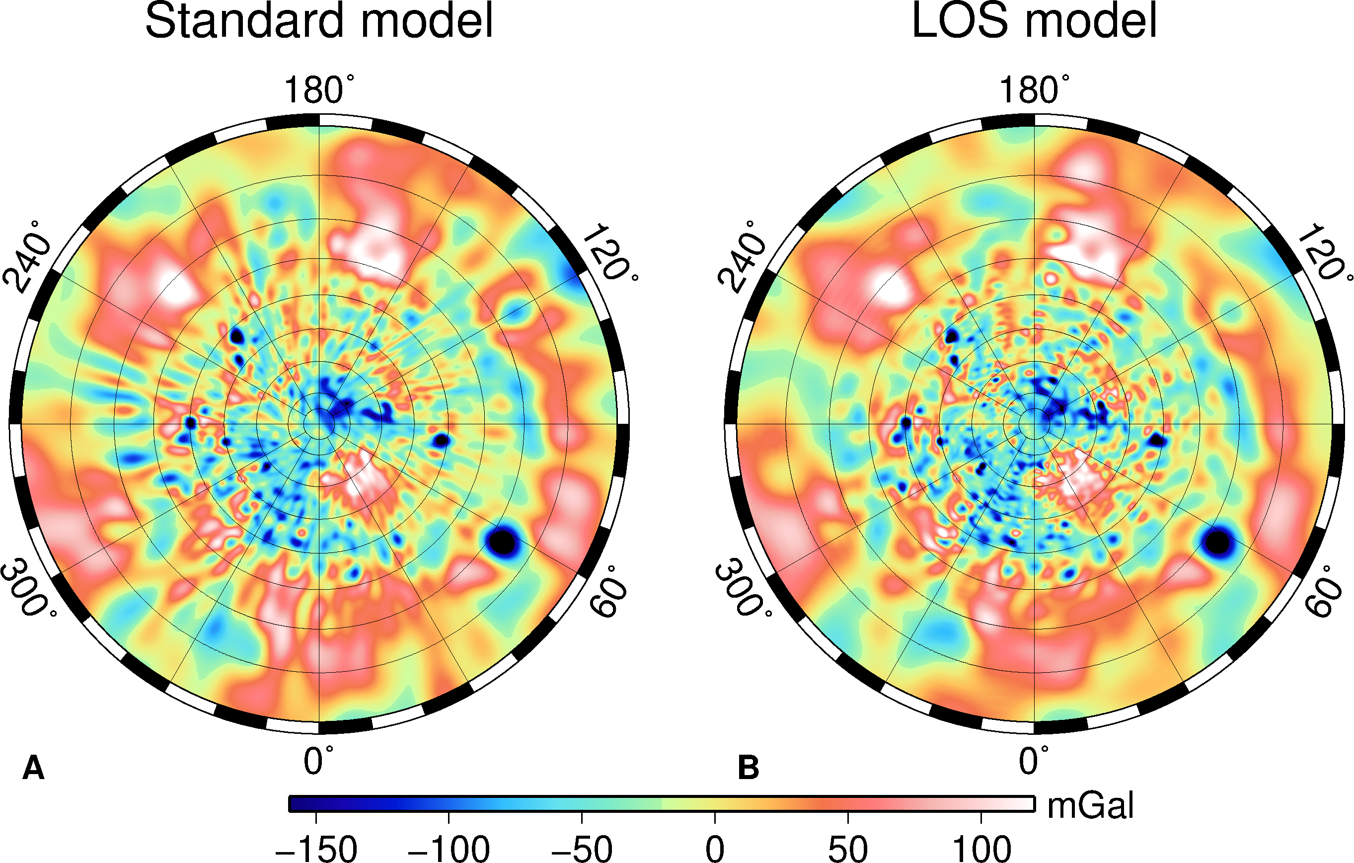
Figure 2. Gravity anomalies for a standard solution based on Doppler data (left,A), and for a solution based on LOS data (right, B). Both solutions are expanded to their maximum degree and order of 180. The maps are in north polar stereographic projection down to 101° N.
We use these models for an analysis of the admittance between gravity and topography, with the goal to determine properties of Mercury's lithosphere. We apply the admittance model of Grott and Wieczorek (2012), and include the equations in the appendix. We select 4 areas where correlations between gravity and topography are high, representing different terrain types: the high-Mg region, the Strindberg crater plus some lobate scarps, heavily cratered terrain, and smooth plains. We employed a Markov Chain Monte Carlo method to estimate crustal density, load density, crustal thickness, elastic thickness, load depth, and a load parameter that describes the ratio between surface and depth loading. We find densities around 2600 kg m-3 for three of the areas, with the density for the fourth area, the northern rise, being higher. The elastic thickness is generally low, between 11 and 30 km.
Data
We present two gravity field models that based on LOS data, one based on standard Doppler data, as well as the results of our admittance analysis.
The difference between the two LOS models is the constraint used to derive them. More details can be found in our paper, but in short, the model indicated as “loose Kaula constraint” is less constrained compared to the other model. We applied this looser constraint because we noted it increases correlations with topography in areas where the spacecraft altitude was low, and it results in flatter admittance spectra. However, care should be taken when using the “loose Kaula” model: it shows spurious signal in many other areas. It should thus be used ONLY in areas where correlations with topography are high.
The files for the gravity field models have the following format:
The first line is a header with comments, starting with "#". The second line has entries GM, ae, lmax, mmax, with GM the gravitational parameter of Mercury, ae the reference radius for this model (2440 km), and lmax and mmax the maximum degree and order, respectively.
All following entries are: degree, order, Clm, Slm, formal error for Clm, formal error for Slm, with Clm and Slm the 4π geodesy normalized spherical harmonics coefficients. The formal errors are computed from the diagonal of the normal matrix.
The files for the admittance analysis contain the results of our MCMC runs to fit the measured admittance to theoretical models. The files contain the parameters for the models that were accepted, as well as the localized theoretical admittance for this model, for the degrees used in the fit (see Table 3 of the paper). The fitted parameters are: crustal density [kg m-3] , load density [kg m-3], crustal thickness [km], elastic thickness [km], load depth [km], and load parameter [no unit]. After that, each line has the entry for localized admittance for that model [mGal/km].
We also provide the measured localized admittance for each area. Entries for these files consist of: degree, admittance, correlation, admittance error, correlation error (the latter is zero by default).
Data Files
Appendix to our paper [PDF].
Gravity field model sha.Doppler: Gravity field model up to degree and order 180 based on Doppler data.
Gravity field model sha.LOS_model : The LOS gravity field model.
Gravity field model sha.LOS_model_loose_constraint : The LOS gravity field model based on a looser constraint, to be used ONLY in areas with high correlations between gravity and topography.
Admittance MCMC results:
Localized admittance for area 1. [loc_admit_area1.out]
Localized admittance for area 2. [loc_admit_area2.out]
Localized admittance for area 3. [loc_admit_area3.out]
Localized admittance for area 4. [loc_admit_area4.out]
MCMC results for area 1 [mcmc_area1.out], with localized theoretical admittance for degrees 30 – 78.
MCMC results for area 2 [mcmc_area2.out], with localized theoretical admittance for degrees 40 – 64.
MCMC results for area 3 [mcmc_area3.out], with localized theoretical admittance for degrees 9 – 32.
MCMC results for area 4 [mcmc_area4.out], with localized theoretical admittance for degrees 9 – 17.
Data Usage Policy
Please cite the following reference when using any of these products:
Goossens et al., 2022, Planet. Sci. J. 3 145, doi:10.3847/PSJ/ac703f
References
Grott, M., and Wieczorek, M.A., 2012, Density and lithospheric structure at Tyrrhena Patera, Mars, from gravity and topography data, Icarus, 221(1), pp. 43-52, doi:10.1016/j.icarus.2012.07.008.