New GRAIL model and a look at crustal density
Sander Goossens
We present updated models of the lunar gravity field using data from the Gravity Recovery and Interior Laboratory (GRAIL) mission (Zuber et al., 2013). These models are expressed in spherical harmonics of degree and order 1200 (an effective resolution at the equator of 4.5 km by 4.5 km). We present models using different constraints: models using a standard Kaula constraint, and models based on a constraint using information from topography. The latter constraint was introduced in Goossens et al. (2017) (see also this PGDA data webpage). The Kaula constraint assumes that spherical harmonic coefficients have a nominal value of 0, and prescribes a variance of K/n2 around that zero value, where K is a constant depending on the planet and n is the degree. As such, the Kaula constraint drives the coefficients to zero. Our topography constraint assigns infinite variance in a chosen direction (called xa, a vector of spherical harmonic coefficients), and the preferred state for all other directions orthogonal to xa is 0, just like the Kaula constraint. In our case, for xa we choose the coefficients from an expansion of gravity from topography, following Wieczorek and Phillips (1998) and using data from the Lunar Orbiter Laser Altimeter (LOLA) onboard the Lunar Reconnaissance Orbiter (LRO) (Smith et al., 2016). This means that there is one degree-of-freedom in our constraint, which is a scale-factor on xa. Our constraint is thus called rank-minus-one, or RM1.
In Goossens et al. (2017) we showed that using this constraint we obtain the correct estimate for the bulk density of the crust using a pre-GRAIL data system. We then applied the constraint to Mars, obtaining an average bulk crustal density lower than generally assumed. Here, we apply this constraint to our latest analysis of the GRAIL data using both primary and extended mission data. We compare the results for this model with those using a standard Kaula constrained model. The Kaula constrained model is called GRGM1200B. The RM1 models are generated with a weight factor λ that indicates how strongly the constraint is applied.
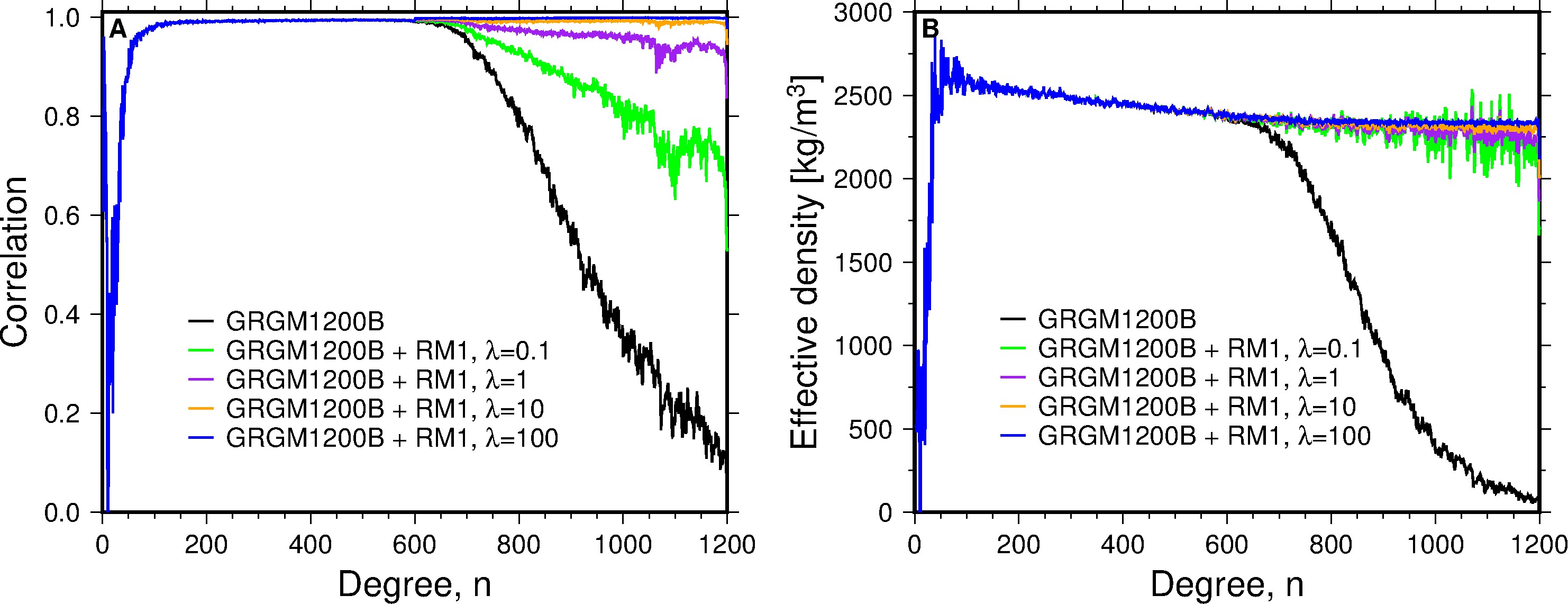
Figure 1. Correlations between gravity and gravity-from-topography (A) and effective density spectrum (B) for the Kaula constrained GRGM1200B model and its RM1 variants.
In Figure 1 we present the correlation between gravity and gravity-from-topography, and the effective density spectrum, an unbiased estimate of the density of the crust per spherical harmonical degree, or in other words, at different spatial scales (for a definition, see Wieczorek et al., 2013). The RM1 constraint improves correlations with topography by design, and it also results in a stable effective density spectrum over the entire degree range of the model, whereas the Kaula constrained model's effective density spectrum collapses. In Figure 2, we show the Bouguer anomalies for GRGM1200B with the RM1 constraint using λ=1, showing smooth anomalies up to degree and order 900.
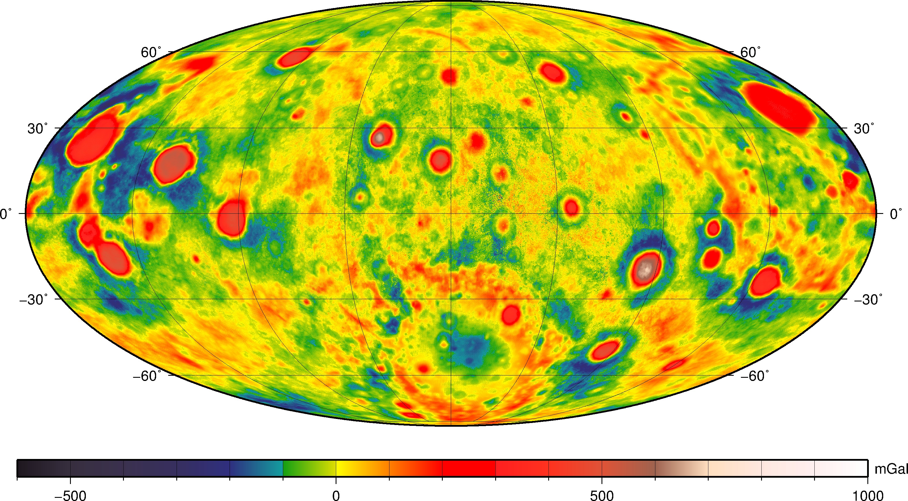
Figure 2. Bouguer anomalies for the RM1 model with λ=1. We used a crustal density of 2500 kg/m3. The Bouguer anomalies were expanded between degrees 7 and 900. The map is in Mollweide projection centered on the farside.
In Goossens et al. (2019), we introduce GRGM1200B and its RM1 variants. We use the RM1 models in an analysis of the lateral and vertical density structure of the lunar crust, based on the earlier study by Besserer et al. (2014). Our RM1 models allow us to extend the resolution of this study.
Here, we provide the spherical harmonic coefficients of the GRGM1200B model and its RM1 variants, as well as additional data sets, such as clones for the models from the covariance, and NetCDF grid files for the maps presented in Goossens et al. (2019). All spherical harmonic files have a straightforward format: the first line contains the model's GM and mean radius value together with the values of the maximum degree and order. All following lines contain entries "degree, order, Clm, Slm, sigma Clm, sigma Slm".
Data
Gravity-model specific data files:
Spherical Harmonic Coefficients for GRGM1200B (the Kaula constrained model). The formal errors on this file have the calibration factor (1.555) as listed in Goossens et al. (2019) applied.-> download the spherical harmonics coefficients of GRGM1200B
Spherical Harmonic Coefficients for GRGM1200B + RM1, for λ = 0.1, 1, 10 and 100. The model for RM1 λ = 100 does not have formal errors included. The formal errors on the other files have the calibration factors applied (1.529, 1.561, and 1.620 for λ = 0.1, 1, and 10, respectively).
-> download the spherical harmonics coefficients of GRGM1200B RM1 for λ = 0.1
-> download the spherical harmonics coefficients of GRGM1200B RM1 for λ = 1
-> download the spherical harmonics coefficients of GRGM1200B RM1 for λ = 10
-> download the spherical harmonics coefficients of GRGM1200B RM1 for λ = 100
A set of 100 clone models (an ensemble of solutions of the same statistical family, see Sabaka et al., 2014) for GRGM1200B, and for the RM1 λ = 0.1, 1, and 10 models. Each set of clone models is in a .tar.gz archive, and its size is about 1.7 GB each (4.2 GB uncompressed).
-> download 100 clones of GRGM1200B
-> download 100 clones of GRGM1200B RM1 for λ = 0.1
-> download 100 clones of GRGM1200B RM1 for λ = 1
-> download 100 clones of GRGM1200B RM1 for λ = 10
Grid file of the Bouguer anomalies for GRGM1200B RM1 λ = 1, for degrees 7-900, using a crustal density of 2500 kg/m3, as shown in Figure 2 here (and Figure 7 of Goossens et al., 2019).
-> download the netCDF/GMT map of Bouguer anomalies of GRGM1200B RM1 for λ = 1
Grid files of anomaly errors (in mGal) for GRGM1200B and GRGM1200B RM1 λ = 1 (Figure 11A and B, respectively, of Goossens et al., 2019).
-> download the netCDF/GMT map of anomaly errors of GRGM1200B
-> download the netCDF/GMT map of anomaly errors of GRGM1200B RM1 for λ = 1
Grid files of degree strength for GRGM1200B and GRGM1200B RM1 λ = 1 (Figure 11C and D, respectively, of Goossens et al., 2019).
-> download the netCDF/GMT map of degree strength of GRGM1200B
-> download the netCDF/GMT map of degree strength of GRGM1200B RM1 for λ = 1
Data files for the analysis of lateral and vertical density variations of the lunar crust:
These are all based on the RM1 model using λ = 10 unless indicated otherwise.Maximum degree values from localized correlations (Figure 12 of Goossens et al., 2019).
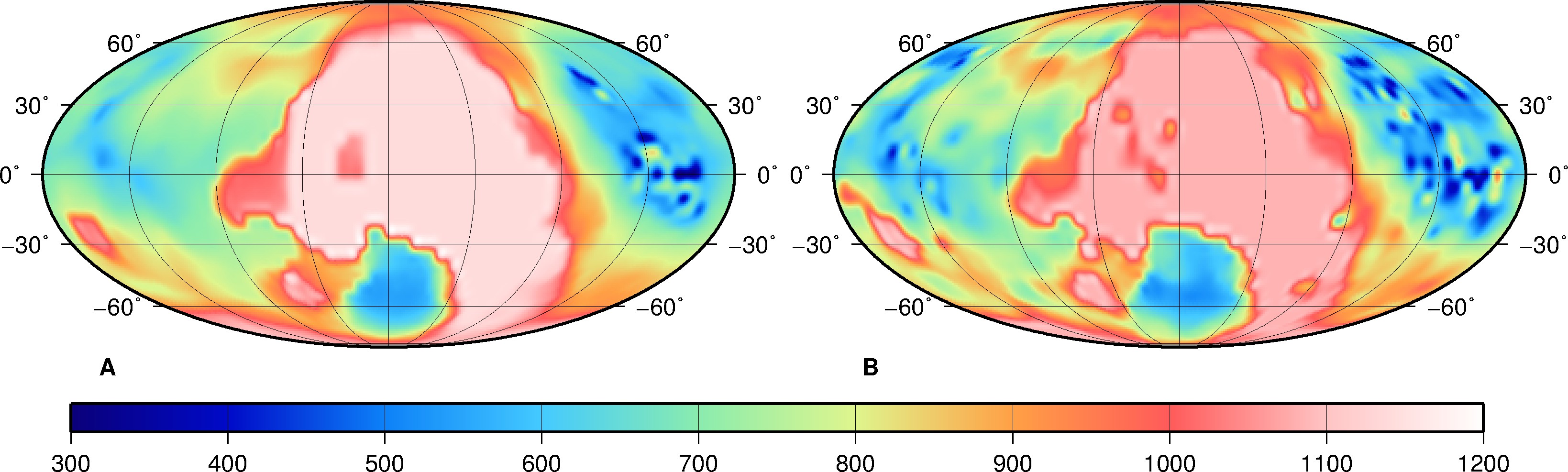
Grid files of maximum degree values, determined as the degree where localized correlations between gravity and gravity-from-topography drop below 0.9. There are grid files for localizations using a cap of 15° (and a spectral bandwidth of 58 for the windowing tapers, Figure A) and for localizations using a cap of 7.5° (with a spectral bandwidth of 116 for the tapers, Figure B).
-> download the netCDF/GMT map of maximum degree for the 15°-cap localization
-> download the netCDF/GMT map of maximum degree for the 7.5°-cap localization
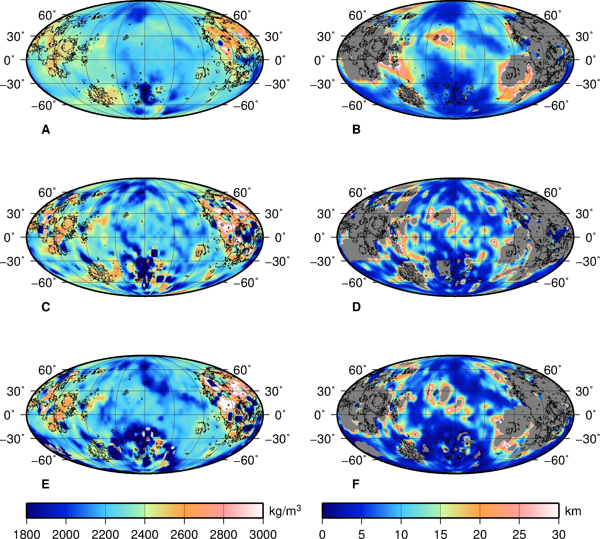
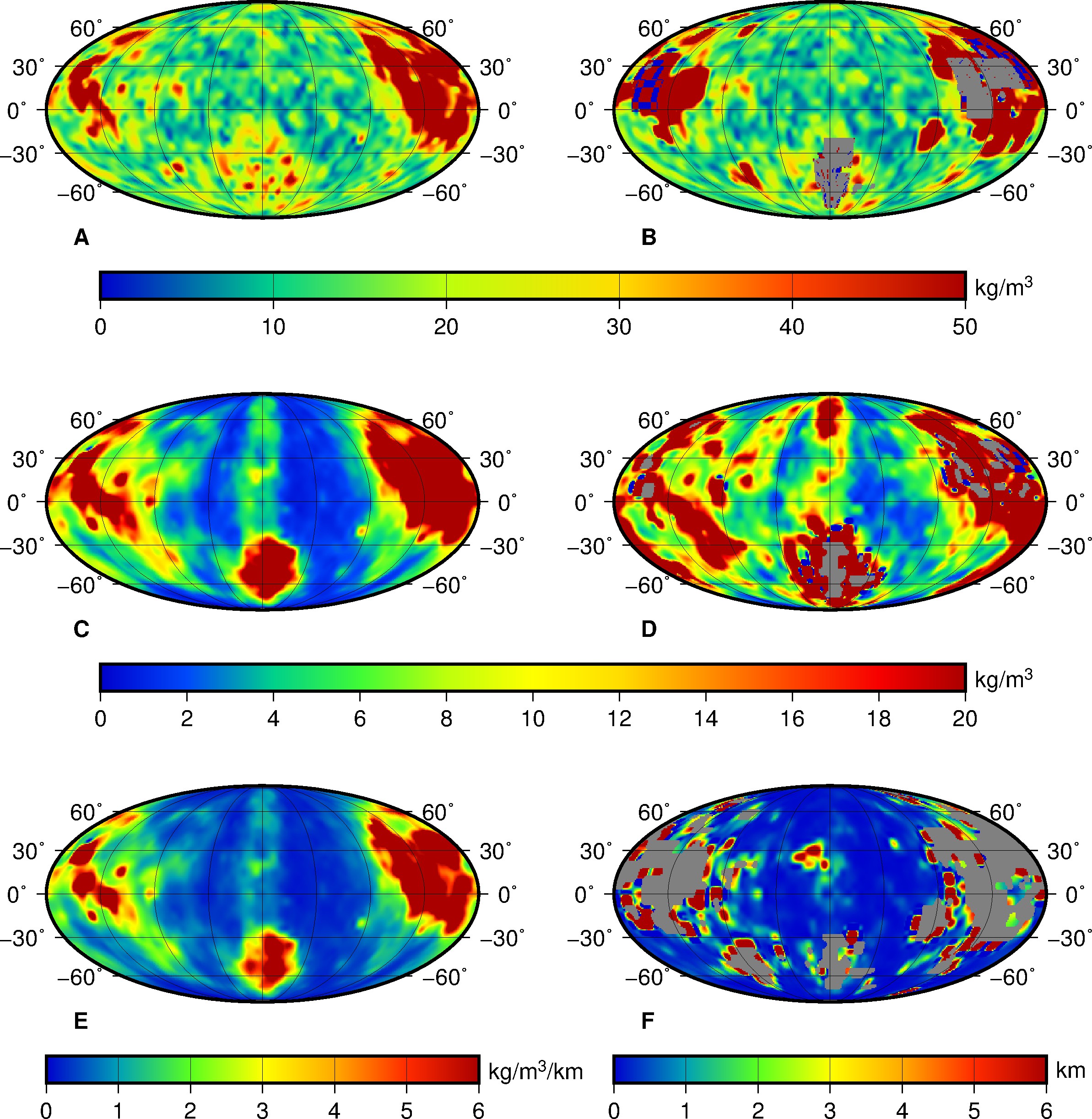
Results for the linear density model (Figure 13 of Goossens et al., 2019).

Grid files for the linear density model for surface density and linear density gradient, for the following cases: using a cap size of 15° for the localizations and a degree range of 250-650 when fitting the models (For the Figure shown here: A for surface density, B for gradient), using a cap size of 7.5° and a degree range of 250-650 (Figure C for surface density, D for gradient), and using a cap size of 7.5° and the variable degree range (as given by the grid files listed above; Figure E for surface density and F for gradient).
-> download the netCDF/GMT map for subpanel A
-> download the netCDF/GMT map for subpanel B
-> download the netCDF/GMT map for subpanel C
-> download the netCDF/GMT map for subpanel D
-> download the netCDF/GMT map for subpanel E
-> download the netCDF/GMT map for subpanel F
Results for the exponential density model (Figure 14 of Goossens et al., 2019).
Grid files for the exponential density model for surface density and e-fold depth, for the following cases: using a cap size of 15° for the localizations and a degree range of 250-650 when fitting the models (For the Figure shown here: A for surface density, B for e-fold depth), using a cap size of 7.5° and a degree range of 250-650 (Figure C for surface density, D for e-fold depth), and using a cap size of 7.5° and the variable degree range (as given by the grid files listed above; Figure E for surface density and F for e-fold depth).
-> download the netCDF/GMT map for subpanel A
-> download the netCDF/GMT map for subpanel B
-> download the netCDF/GMT map for subpanel C
-> download the netCDF/GMT map for subpanel D
-> download the netCDF/GMT map for subpanel E
-> download the netCDF/GMT map for subpanel F
Results for linear and exponential density models using the RM1 λ = 1 model (Figure 17 of Goossens et al., 2019).

Grid files for the linear and exponential models for the RM1 λ = 1 model: for the linear model, surface density (Figure A) and linear gradient (Figure B), and for the exponential model, surface density (Figure C) and e-fold depth (Figure D). Note that Figure 17 of Goossens et al. (2019) shows the density differences instead of gradient and e-fold depth.
-> download the netCDF/GMT map for subpanel A
-> download the netCDF/GMT map for subpanel B
-> download the netCDF/GMT map for subpanel C
-> download the netCDF/GMT map for subpanel D
Results of an error analysis of the density results (Figure 18 of Goossens et al., 2019).
Grid files for the misfit of the effective density spectra (Figure A for the linear model, B for the exponential model), and of the errors in surface density (Figure C for the linear model, D for the exponential model) and gradients (Figure E for the linear gradient and F for the e-fold depth). The error analysis was performed with clone models.
-> download the netCDF/GMT map for subpanel A
-> download the netCDF/GMT map for subpanel B
-> download the netCDF/GMT map for subpanel C
-> download the netCDF/GMT map for subpanel D
-> download the netCDF/GMT map for subpanel E
-> download the netCDF/GMT map for subpanel F
Surface porosity (Figure 19 of Goossens et al., 2019).
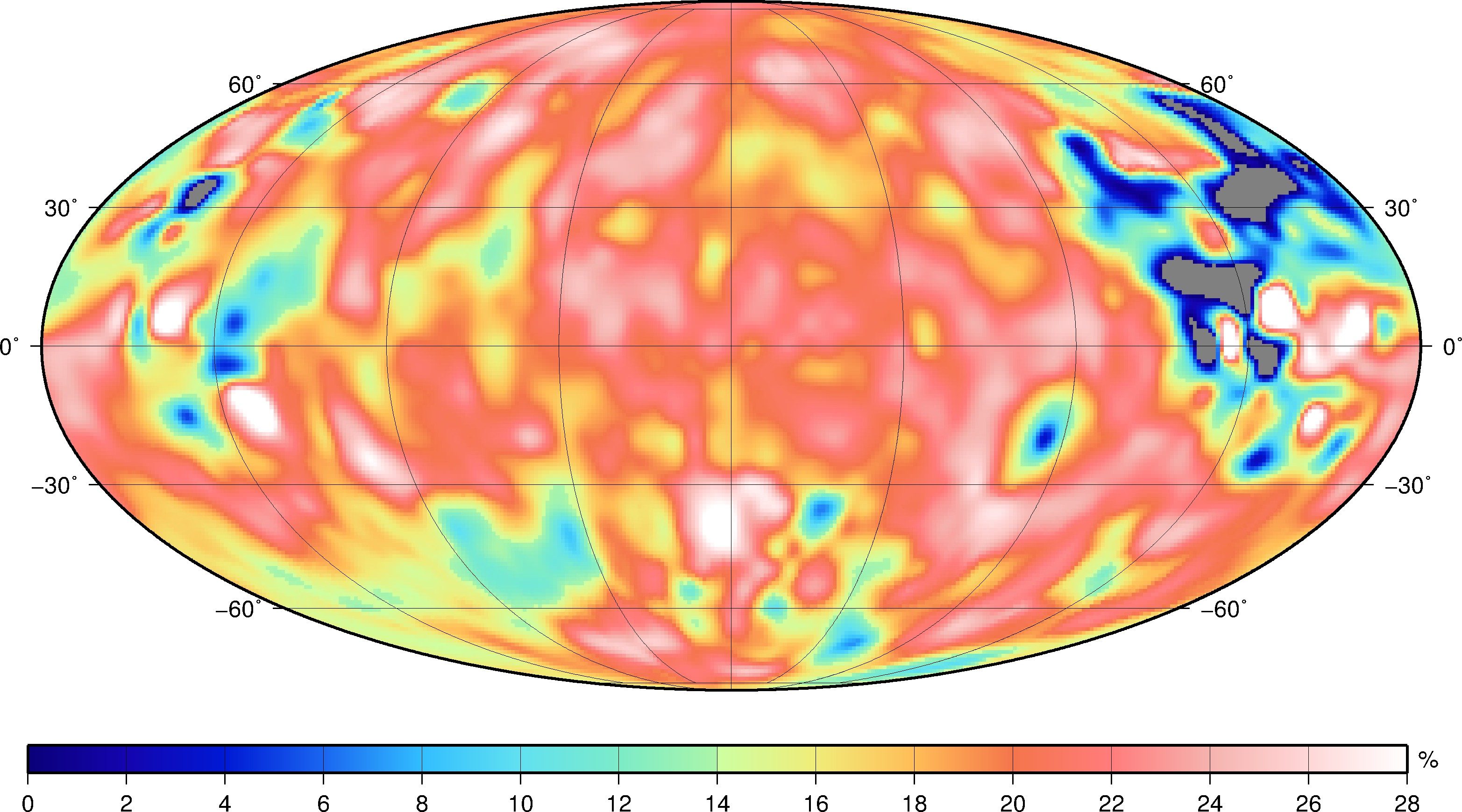
Grid file for the surface porosity, using the results of the linear model with a localization cap size of 7.5° and a degree range of 250-650 in the least-squares fit. To compute the porosity, we used the grain density from Huang and Wieczorek (2012); this can be found at the GRAIL crustal thickness archive (Wieczorek, 2012).
-> download the netCDF/GMT map of porosity
Data Usage Policy
Please cite the following reference when using any of the products described above:Goossens, S., Sabaka, T.J., Wieczorek, M.A., Neumann, G.A., Mazarico, E., Lemoine, F., Nicholas, J.B., Smith, D.E., Zuber, M.T. (2020). High-resolution gravity field models from GRAIL data and implications for models of the density structure of the Moon's crust, Journal of Geophysical Research: Planets, 125, e2019JE006086, doi:10.1029/2019JE006086.
References
[1] Besserer, J., Nimmo, F., Wieczorek, M.A., Weber, R.C., Kiefer, W.S., McGovern, P.J., Andrews?Hanna, J.C., Smith, D.E., Zuber, M.T. (2014), GRAIL gravity constraints on the vertical and lateral density structure of the lunar crust, Geophysical Research Letters, 41, pp. 5771-5777, doi:10.1002/2014GL060240.
[2] Goossens, S., Sabaka, T. J., Genova, A., Mazarico, E., Nicholas, J. B., Neumann, G. A. (2017), Evidence for a low bulk crustal density for Mars from gravity and topography, Geophysical Research Letters, 44 , pp. 7686-7694, doi:10.1002/2017GL074172.
[3] Huang, Q., Wieczorek, M. A. (2012), Density and porosity of the lunar crust from gravity and topography. Journal of Geophysical Research: Planets, 117 (E5), E05003, doi:10.1029/2012JE004062.
[4] Sabaka, T. J., Nicholas, J. B., Goossens, S., Lemoine, F. G., Mazarico, E. (2014), Error propagation for high-degree gravity models developed from the GRAIL mission, retrieved from the PDS.
[5] Smith, D. E., Zuber, M. T., Neumann, G. A., Mazarico, E., Lemoine, F. G., III, J. W. H., Lucey, P. G., Aharonson, O., Robinson, M. S., Sun, X., Torrence, M. H., Barker, M. K., Oberst, J., Duxbury, T. C., d. Mao, D., Barnouin, O. S., Jha, K., Rowlands, D. D., Goossens, S., Baker, D., Bauer, S., Gläser,P., Lemelin, M., Rosenburg, M., Sori, M. M., Whitten, J., McClanahan, T. (2016), Summary of the results from the Lunar Orbiter Laser Altimeter after seven years in orbit. Icarus, 283, pp. 70-91, doi:10.1016/j.icarus.2016.06.006.
[6] Wieczorek, M. A., Phillips, R. J. (1998), Potential anomalies on a sphere: Applications to the thickness of the lunar crust, Journal of Geophysical Research, 103 (E1), pp. 1715-1724, doi:10.1029/97JE03136.
[7] Wieczorek, Mark. (2012). GRAIL Crustal Thickness Archive [Data set]. Zenodo, doi:10.5281/zenodo.997347.
[8] Wieczorek, M. A., Neumann, G.A., Nimmo, F., Kiefer, W.S., Taylor, G.J., Melosh, H.J., Phillips, R.J., Solomon, S.C., Andrews-Hanna, J.C., Asmar, S.W., Konopliv, A.S., Lemoine, F.G., Smith, D.E., Watkins, M.M., Williams, J.G., and Zuber, M.T., (2013), The Crust of the Moon as Seen by GRAIL, Science, 339(6120), 671–675, doi:10.1126/science.1231530.
[9] Zuber, M. T., Smith, D. E., Watkins, M. M., Asmar, S. W., Konopliv, A. S., Lemoine, F. G., Melosh, H. J., Neumann, G. A., Phillips, R. J., Solomon, S. C., Wieczorek, M. A., Williams, J. G., Goossens, S. J., Kruizinga, G.,Mazarico, E., Park, R. S., Yuan, D.-N. (2013), Gravity field of the Moon from the Gravity Recovery and Interior Laboratory (GRAIL) mission, Science, 339, pp. 668-671, doi:10.1126/science.1231507.